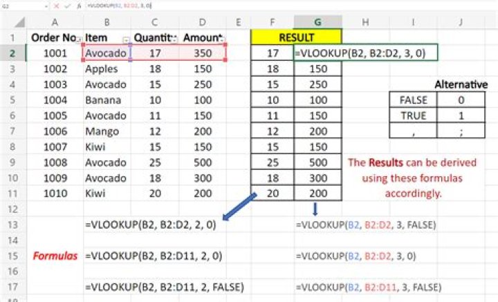
How to Use VLOOKUP in Excel
- Identify a column of cells you'd like to fill with new data.
- Select 'Function' (Fx) > VLOOKUP and insert this formula into your highlighted cell.
- Enter the lookup value for which you want to retrieve new data.
- Enter the table array of the spreadsheet where your desired data is located.
Similarly one may ask, how do I populate multiple cells using Vlookup?
3 Answers
- Select the cells (cells equal to the number of columns that you wish to fetch) where you wish to populate the VLOOKUP results.
- Next, without clicking anywhere else type the formula: VLOOKUP("Florian",A:D,{1,2,3,4},FALSE) in the Formula bar.
- After this simply hit the Ctrl + Shift + Enter keys.
Similarly, can you use Vlookup in data validation? The VLOOKUP function in Excel can become interactive and more powerful when applying a Data Validation (drop down menu/list) as the Lookup_Value. So as you change your selection from the drop down list, the VLOOKUP value also changes. For the Source, ensure that it has the 4 Stock List values selected. Click OK.
Subsequently, one may also ask, how do I populate data in Excel based on another cell?
Fill data automatically in worksheet cells
- Select one or more cells you want to use as a basis for filling additional cells. For a series like 1, 2, 3, 4, 5, type 1 and 2 in the first two cells. For the series 2, 4, 6, 8, type 2 and 4.
- Drag the fill handle .
- If needed, click Auto Fill Options. and choose the option you want.
How do I AutoFill data validation list?
AutoComplete for Data Validation List
- Go to Tools>Options - Edit and check Enable AutoComplete for cell values.
- Move your list of items is in the range immediately above the Validation cell.
- Hide the rows above your Validation cell.
Related Question Answers
How do you auto populate cells from another sheet in Excel?
Go to Sheet2, click in cell A1 and click on the drop-down arrow of Paste button on the Home tab and select Paste Link button. It will generate a link by automatically entering the formula =Sheet1! A1 .How do I create an AutoFill form in Excel?
How to create an efficient AutoFill series in Excel- Enter the values and then select the list.
- Choose Options from the Tools menu.
- Click the Custom Lists tab.
- Click Import.
- Click OK to return to the sheet.
- Select a blank cell, enter the first item in the list and then expand the fill handle to complete the list.
How do I drag down a Vlookup formula?
To copy the formula down a column, we need to follow these steps:- Select cell C3 and click on it.
- Insert the formula: =VLOOKUP(B3,$E$3:$F$7,2,0)
- Press enter.
- Drag the formula down to the other cells in the column by clicking and dragging the little “+” icon at the bottom-right of the cell.
How do I do a Vlookup for all rows?
To get the whole row data of a matched value, please apply the following formula: Enter this formula: =VLOOKUP($F$2,$A$1:$D$12,COLUMN(A1),FALSE) into a blank cell where you want to get the result, for instance, H1, and then drag the formula to right ( from H2 to K2), and you will get the whole row data you want.How do you autofill multiple cells in Excel?
Type the data into a spreadsheet cell. Place the cursor in the bottom right corner of the cell you just typed in until you see a plus sign. With the left mouse button, press and drag the Fill Handle (plus sign) to highlight all of the cells you want filled.How do I copy and paste a Vlookup formula in Excel?
Just use the old good copy & paste way:- Click the cell with the formula to select it.
- Press Ctrl + C to copy the formula.
- Select a cell or a range of cells where you want to paste the formula (to select non-adjacent ranges, press and hold the Ctrl key).
- Press Ctrl + V to paste the formula.
How do I Vlookup multiple values horizontally?
To get the multiple corresponding values horizontally, in one row, just make one change in the formula, by replacing "ROW(1:1)" to "COLUMN(A1)", and then copy the formula horizontally in the same row to the right columns, from Cell B11 to H11, in 7 columns (Refer Table 6).How do you do a Vlookup when the same value is repeated?
If it is returning the same value over and over again for your whole range, you probably have your Calculation Options set to "Manual". Go into Formulas on the top ribbon and choose Calculation Options. There, you can change your calc method to "Automatic".Can I do a Vlookup across multiple columns?
I showed these users a quicker way to create VLookUps across multiple columns with just a small change to a standard VLookUp.- Step 1 – Column Index Numbers.
- Step 2 – First VLookUp.
- Step 3 – Make LookUp Value Column Absolute.
- Step 4 – Make Table Array Absolute.
- Step 5 – Update Column Index Number.
Where is AutoFill in Excel?
Put the mouse pointer over the bottom right-hand corner of the cell until it's a black plus sign. Click and hold the left mouse button, and drag the plus sign over the cells you want to fill. And the series is filled in for you automatically using the AutoFill feature.How do I copy a formula to an entire column?
Select the cell with the formula and the adjacent cells you want to fill. Click Home > Fill, and choose either Down, Right, Up, or Left. Keyboard shortcut: You can also press Ctrl+D to fill the formula down in a column, or Ctrl+R to fill the formula to the right in a row.How do you copy a Vlookup without formula?
Just follow these steps.- Select the cells or ranges you wish to copy.
- Select the “Home” tab.
- Select “Copy” in the “Clipboard section.
- Select the cell you wish to paste your values to.
- Select the lower half of the large “Paste” button. From the extended menu that appears, select “Values“.
- Select “OK“.