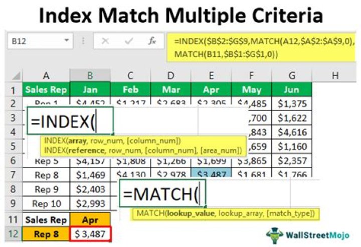
- Step 1: Understanding the foundation.
- Step 2: Insert a normal MATCH INDEX formula.
- Step 3: Change the lookup value to 1.
- Step 4: Enter the criteria.
- Step 5: Ctrl + Shift + Enter.
Then, can index match pull multiple values?
This is an array formula and must be entered with Control + Shift + Enter. The SMALL function returns each matching row number, which is supplied to the INDEX function as row_num, with the named range "names" as the array.
Additionally, how does an index match formula work? The INDEX MATCH formula is the combination of two functions in Excel. CFI's resources are the best way to learn Excel on your own terms.: INDEX and MATCH. =INDEX() returns the value of a cell in a table based on the column and row number. =MATCH() returns the position of a cell in a row or column.
Also know, how can I get multiple matching values in Excel?
Pull rows with multiple matches to the main table
- Select your main table or click any cell within it, and then click the Merge Two Tables button on the ribbon:
- The add-in is smart enough to identify and pick the entire table, so you just click Next:
- Select the lookup table, and click Next.
Can you do index match match match?
In many cases, merging data in Excel can easily be accomplished with a single INDEX-MATCH (or a VLOOKUP). Sometimes, though, it's time to bring out the big guns — the INDEX-MATCH-MATCH. The INDEX-MATCH-MATCH combines two MATCH statements into the row and column positions in an INDEX formula.
Related Question Answers
How do you lookup multiple values?
How to Perform VLOOKUP for Multiple Criteria Using the Array Formula- Click on the VLOOKUP-Arrays worksheet tab in the VLOOKUP advanced sample file.
- Type the SUM-VLOOKUP formula in cell H3:
- Click Ctrl+Shift+Enter on your keyboard to add the curly brackets:
Can Xlookup return multiple values?
One more amazing feature of XLOOKUP is its ability to return more than one value relating to the same match. All is done with the standard syntax and without any extra manipulations! You enter the formula in the top-left cell of the results range, and Excel automatically spills the results into adjacent blank cells.How do I return multiple values in one cell?
Vlookup to return multiple values into one cell with a useful feature- Select the data range that you want to combine one column data based on another column.
- Click Kutools > Merge & Split > Advanced Combine Rows, see screenshot:
- In the popped out Advanced Combine Rows dialog box:
Does index match return first value?
If matched, the adjacent values in Column C should be returned. However, if Column A has a value which is repeated, the INDEX/MATCH function returns the first value from Column B rather than the 2nd or 3rd value being looked-up in Column B.Why is index and match better than Vlookup?
With unsorted data, VLOOKUP and INDEX-MATCH have about the same calculation times. That is, INDEX-MATCH is only about 3% faster. With sorted data and an approximate match, INDEX-MATCH is about 30% faster than VLOOKUP. If you use VLOOKUP you must look up the same SKU for each column of information you need.Can you index match multiple columns?
Normally, an INDEX MATCH formula is configured with MATCH set to look through a one-column range and provide a match based on given criteria. Without concatenating values in a helper column, or in the formula itself, there's no way to supply more than one criteria.Why does my index match not work?
If you believe that the data is present in the spreadsheet, but MATCH is unable to locate it, it may be because: The cell has unexpected characters or hidden spaces. The cell may not be formatted as a correct data type. For example, the cell has numerical values, but it may be formatted as Text.How do I filter multiple values in Excel?
To filter with search:- Select the Data tab, then click the Filter command. A drop-down arrow will appear in the header cell for each column.
- Click the drop-down arrow for the column you want to filter.
- The Filter menu will appear.
- When you're done, click OK.
- The worksheet will be filtered according to your search term.
How do I list all matching values in Excel?
In the Formulas Helper dialog box, you need to: 2.1 Find and select Look for a value in list option in the Choose a formula box; Tips: You can check the Filter box, enter the keyword into the textbox to quickly filter the formula you need.Can you do multiple VLOOKUPs in one formula?
By nesting multiple VLOOKUPs inside the IFERROR function, the formula allows for sequential lookups. If the first VLOOKUP fails, IFERROR catches the error and runs another VLOOKUP. If the second VLOOKUP fails, IFERROR catches the error and runs another VLOOKUP, and so on.How do I extract multiple rows from matching criteria in Excel?
This is an array formula and must be entered with Control + Shift + Enter. After you enter the formula in the first cell, drag it down and across to fill in the other cells.How do I match data and return values in Excel?
In the Formula Type drop down list, please select Lookup option; Then, select Look for a value in list option in the Choose a formula list box; And then, in the Arguments input text boxes, select the data range, criteria cell and column you want to return matched value from separately.How do you calculate the index?
To calculate the Price Index, take the price of the Market Basket of the year of interest and divide by the price of the Market Basket of the base year, then multiply by 100.How do I use index match with Sumif?
- We can meet our objectives by nesting the INDEX and MATCH functions inside of our SUMIFS function to dynamically select the proper sum column.
- One approach is to use the INDEX/MATCH functions.
- The INDEX function can actually return a cell value or a range reference.
Can you use index match horizontal?
This is because INDEX and MATCH is incredibly flexible – you can do horizontal and vertical lookups, 2-way lookups, left lookups, case-sensitive lookups, and even lookups based on multiple criteria. If you want to improve your Excel skills, INDEX and MATCH should be on your list.What is the difference between Vlookup and index match?
The key difference between INDEX MATCH and VLOOKUP is that VLOOKUP requires a static column reference while INDEX MATCH uses a dynamic column reference. With VLOOKUP, most people will input a specific, static number to indicate which column they want to return from.How do you do Xlookup?
Syntax. The XLOOKUP function searches a range or an array, and returns an item corresponding to the first match it finds. If a match doesn't exist, then XLOOKUP can return the closest (approximate) match. Where a valid match is not found, return the [if_not_found] text you supply.How do I use index and match instead of Vlookup?
VLOOKUP is prone to error, especially in big spreadsheets- With VLOOKUP, you specify a number to represent which column you want to return the value from. So you have count the columns to figure out which one you want.
- With INDEX MATCH, you select the specific column of data from which you want to return the value.
What is index function in Excel?
The INDEX function returns a value or the reference to a value from within a table or range. There are two ways to use the INDEX function: If you want to return the value of a specified cell or array of cells, see Array form. If you want to return a reference to specified cells, see Reference form.How do I do an IF match in Excel?
The MATCH function searches for a specified item in a range of cells, and then returns the relative position of that item in the range. For example, if the range A1:A3 contains the values 5, 25, and 38, then the formula =MATCH(25,A1:A3,0) returns the number 2, because 25 is the second item in the range.How do I nest a match function?
INDEX and MATCH are “nested” functions – two functions used together. The first argument of INDEX is to give it an array. This array (range) should include your answer. You then need to specify how many rows to go down and how many columns to move to find the correct value.Can you do index match with 3 criteria?
- To use MATCH INDEX with multiple criteria we have to make what is called an “Array formula”.
- The lookup array tells Excel where you want the MATCH function to look for the lookup value.
- Now your formula should look like this: